How to write a custom scan handling for specplot
Sometimes, it will be obvious that a certain scan macro never generates any plot images, or that the default handling creates a plot that is a poor representation of the data, such as the hklscan where only one of the the axes hkl is scanned. To pick the scanned axis for plotting, it is necessary to prepare custom handling and replace the default handling.
Overview
It is possible to add in additional handling by writing a Python module.
This module creates a subclass of the standard handling, such as
LinePlotter,
MeshPlotter, or their superclass
ImageMaker.
The support is added to the macro selection class
Selector with code such as in the brief
example described below: Change the plot title text in ascan macros:
selector = spec2nexus.specplot.Selector()
selector.add('ascan', Custom_Ascan)
spec2nexus.specplot_gallery.main()
Data Model
The data to be plotted is kept in an appropriate subclass
of PlotDataStructure in attributes
show in the next table. The data model is an adaptation of the
NeXus NXdata base class. [1]
| attribute | description |
|---|---|
| self.signal | name of the dependent data (y axis or image) to be plotted |
| self.axes | list of names of the independent axes [2] |
| self.data | dictionary with the data, indexed by name |
| [1] | NeXus NXdata base class: http://download.nexusformat.org/doc/html/classes/base_classes/NXdata.html |
| [2] | The number of names provided in self.axes is equal to the rank of the signal data (self.data[self.signal]). For 1-D data, self.axes has one name and the signal data is one-dimensional. For 2-D data, self.axes has two names and the signal data is two-dimensional. |
Steps
In all cases, custom handling of a specific SPEC macro name is provided by
creating a subclass of ImageMaker and defining
one or more of its methods. In the simplest case, certain settings may be
changed by calling spec2nexus.specplot.ImageMaker.configure() with
the custom values. Examples of further customization are provided below, such
as when the data to be plotted is stored outside of the SPEC data file. This
is common for images from area detectors.
It may also be necessary to create a subclass
of PlotDataStructure to gather the data to be plotted
or override the default spec2nexus.specplot.ImageMaker.plottable() method.
An example of this is shown with the MeshPlotter and
associated MeshStructure classes.
Examples
A few exmaples of custom macro handling are provided, some simple, some complex. In each example, decisions have been made about where to provide the desired features.
Change the plot title text in ascan macros
The SPEC ascan macro is a workhorse and records the scan
of a positioner and the measurement of data in a counter.
Since this macro name ends with “scan”, the default selection
in specplot images this data
using the LinePlotter class.
Here is a plot of the default handling of data from the ascan macro:
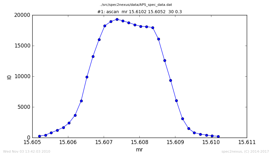
Standard plot of data from ascan macro
We will show how to change the plot title as a means to illustrate how to customize the handling for a scan macro.
We write Custom_Ascan which is a subclass of
LinePlotter. The get_plot_data method is written
(overrides the default method) to gain access to the place
where we can introduce the change. The change is made by the call to
the configure method (defined in the superclass). Here’s the code:
ascan.py example
1 2 3 4 5 6 7 8 9 10 11 12 13 14 15 16 17 18 19 20 21 22 23 24 25 26 27 28 29 30 31 32 33 34 35 36 37 38 39 40 41 | #!/usr/bin/env python
#-----------------------------------------------------------------------------
# :author: Pete R. Jemian
# :email: prjemian@gmail.com
# :copyright: (c) 2014-2020, Pete R. Jemian
#
# Distributed under the terms of the Creative Commons Attribution 4.0 International Public License.
#
# The full license is in the file LICENSE.txt, distributed with this software.
#-----------------------------------------------------------------------------
'''
Plot all scans that used the SPEC `ascan` macro, showing only the scan number (not full scan command)
This is a simple example of how to customize the scan macro handling.
There are many more ways to add complexity.
'''
import spec2nexus.specplot
import spec2nexus.specplot_gallery
class Custom_Ascan(spec2nexus.specplot.LinePlotter):
'''simple customization'''
def retrieve_plot_data(self):
'''substitute with the data&time the plot was created'''
import datetime
spec2nexus.specplot.LinePlotter.retrieve_plot_data(self)
self.set_plot_subtitle(str(datetime.datetime.now()))
def main():
selector = spec2nexus.specplot.Selector()
selector.add('ascan', Custom_Ascan)
spec2nexus.specplot_gallery.main()
if __name__ == '__main__':
main()
|
See the changed title:
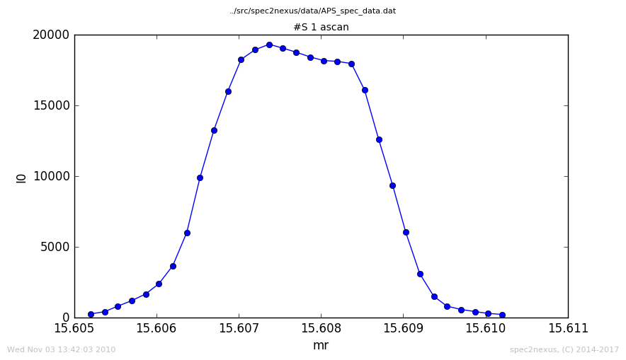
Customized plot of data from ascan macro
Make the y-axis log scale
A very simple customization can make the Y axis to be logarithmic scale. (This customization is planned for an added feature [3] in a future relase of the spec2nexus package.) We present two examples.
modify handling of a2scan
One user wants all the a2scan images to be plotted with a logarithmic scale on the Y axis. Here’s the code:
custom_a2scan_gallery.py example
1 2 3 4 5 6 7 8 9 10 11 12 13 14 15 16 17 18 19 20 21 22 23 24 25 26 27 28 29 30 31 32 33 34 35 36 37 38 39 40 41 42 43 44 45 46 47 48 49 50 51 52 53 54 55 56 57 58 59 60 61 62 63 64 | #!/usr/bin/env python
'''
Customization for specplot_gallery: plot a2scan with log(y) axis
This program changes the plotting for all scans that used the *a2scan* SPEC macro.
The Y axis of these plots will be plotted as logarithmic if all the data values are
greater than zero. Otherwise, the Y axis scale will be linear.
'''
import spec2nexus.specplot
import spec2nexus.specplot_gallery
class Custom_a2scan_Plotter(spec2nexus.specplot.LinePlotter):
'''plot `a2scan` y axis as log if possible'''
def retrieve_plot_data(self):
'''plot the vertical axis on log scale'''
spec2nexus.specplot.LinePlotter.retrieve_plot_data(self)
choose_log_scale = False
if self.signal in self.data: # log(y) if all data positive
choose_log_scale = min(self.data[self.signal]) > 0
self.set_y_log(choose_log_scale)
def main():
selector = spec2nexus.specplot.Selector()
selector.add('a2scan', Custom_a2scan_Plotter)
spec2nexus.specplot_gallery.main()
if __name__ == '__main__':
# debugging_setup()
main()
'''
Instructions:
Save this file in a directory you can write and call it from your cron tasks.
Note that in cron entries, you cannot rely on shell environment variables to
be defined. Best to spell things out completely. For example, if your $HOME
directory is `/home/user` and you have these directories:
* `/home/user/bin`: various custom executables you use
* `/home/user/www/specplots`: a directory you access with a web browser for your plots
* `/home/user/spec/data`: a directory with your SPEC data files
then save this file to `/home/user/bin/custom_a2scan_gallery.py` and make it executable
(using `chmod +x ./home/user/bin/custom_a2scan_gallery.py`).
Edit your list of cron tasks using `crontab -e` and add this (possibly
replacing a call to `specplot_gallery` with this call `custom_a2scan_gallery.py`)::
# every five minutes (generates no output from outer script)
0-59/5 * * * * /home/user/bin/custom_a2scan_gallery.py -d /home/user/www/specplots /home/user/spec/data 2>&1 >> /home/user/www/specplots/log_cron.txt
Any output from this periodic task will be recorded in the file
`/home/user/www/specplots/log_cron.txt`. This file can be reviewed
for diagnostics or troubleshooting.
'''
|
custom uascan
The APS USAXS instrument uses a custom scan macro called uascan for routine step scans.
Since this macro name ends with “scan”, the default selection in specplot images this data
using the LinePlotter class.
Here is a plot of the default handling of data from the uascan macro:
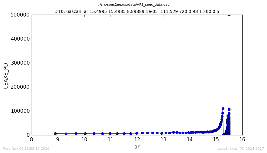
USAXS uascan, handled as LinePlotter
The can be changed by making the y axis log scale.
To do this, a custom version of LinePlotter
is created as Custom_Ascan. The get_plot_data method is written
(overrides the default method) to make the y axis log-scale by calling
the configure method (defined in the superclass). Here’s the code:
usaxs_uascan.py example
1 2 3 4 5 6 7 8 9 10 11 12 13 14 15 16 17 18 19 20 21 22 23 24 25 26 27 28 29 30 31 32 33 34 35 36 37 38 39 40 41 42 43 44 45 46 47 48 49 50 51 52 53 54 55 56 57 58 59 60 61 62 63 64 65 66 67 | #!/usr/bin/env python
#-----------------------------------------------------------------------------
# :author: Pete R. Jemian
# :email: prjemian@gmail.com
# :copyright: (c) 2014-2017, Pete R. Jemian
#
# Distributed under the terms of the Creative Commons Attribution 4.0 International Public License.
#
# The full license is in the file LICENSE.txt, distributed with this software.
#-----------------------------------------------------------------------------
'''
Plot data from the USAXS uascan macro
.. autosummary::
~UAscan_Plotter
'''
import spec2nexus.specplot
import spec2nexus.specplot_gallery
class UAscan_Plotter(spec2nexus.specplot.LinePlotter):
'''simple customize of `uascan` handling'''
def retrieve_plot_data(self):
'''plot the vertical axis on log scale'''
spec2nexus.specplot.LinePlotter.retrieve_plot_data(self)
if self.signal in self.data:
if min(self.data[self.signal]) <= 0:
# TODO: remove any data where Y <= 0 (can't plot on log scale)
msg = 'cannot plot Y<0: ' + str(self.scan)
raise spec2nexus.specplot.NotPlottable(msg)
# in the uascan, a name for the sample is given in `self.scan.comments[0]`
self.set_y_log(True)
self.set_plot_subtitle(
'#%s uascan: %s' % (str(self.scan.scanNum), self.scan.comments[0]))
def debugging_setup():
import os, sys
import shutil
import ascan
selector = spec2nexus.specplot.Selector()
selector.add('ascan', ascan.Custom_Ascan) # just for the demo
path = '__usaxs__'
shutil.rmtree(path, ignore_errors=True)
os.mkdir(path)
sys.argv.append('-d')
sys.argv.append(path)
sys.argv.append(os.path.join('..', 'src', 'spec2nexus', 'data', 'APS_spec_data.dat'))
def main():
selector = spec2nexus.specplot.Selector()
selector.add('uascan', UAscan_Plotter)
spec2nexus.specplot_gallery.main()
if __name__ == '__main__':
# debugging_setup()
main()
|
Note that in the uascan, a name for the sample provided by the user is given in self.scan.comments[0]. The plot title is changed to include this and the scan number. The customized plot has a logarithmic y axis:
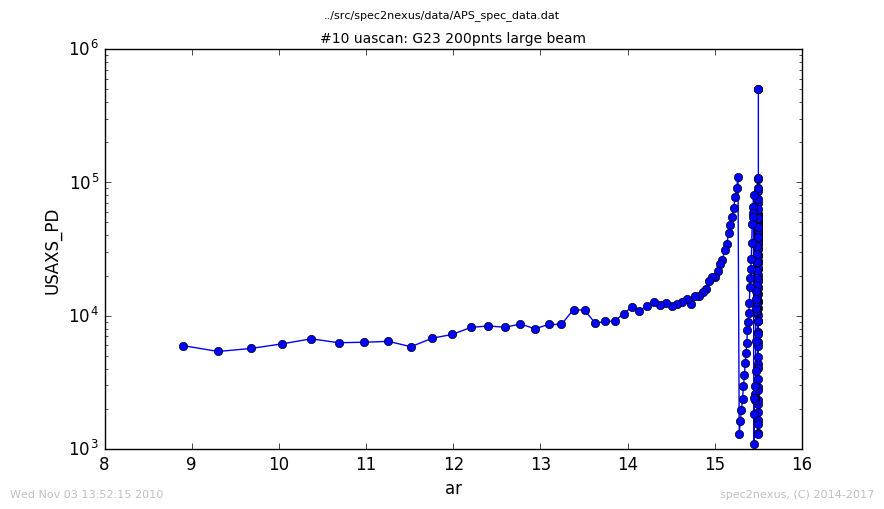
USAXS uascan, with logarithmic y axis
The most informative view of this data is when the raw data are reduced to \(I(Q)\) and viewed on a log-log plot, but that process is beyond this simple example. See the example Get xy data from HDF5 file below.
| [3] | specplot: add option for default log(signal) |
SPEC’s hklscan macro
The SPEC hklscan macro appears in a SPEC data file due to either a hscan, kscan, or lscan. In each of these one of the hkl vectors is scanned while the other two remain constant.
The normal handling of the ascan macro plots the last data column against the first. This works for data collected with the hscan. For kscan or lscan macros, the h axis is still plotted by default since it is in the first column.
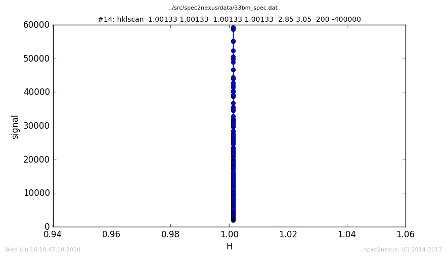
SPEC hklscan (lscan, in this case), plotted against the (default) first axis H
To display the scanned axis, it is necessary to examine the data in a custom
subclass of LinePlotter. The
HKLScanPlotter subclass,
provided with specplot, defines the get_plot_data() method
determines the scanned axis, setting it by name:
plot.axes = [axis,]
self.scan.column_first = axis
Then, the standard plot handling used by LinePlotter uses this information to make the plot.
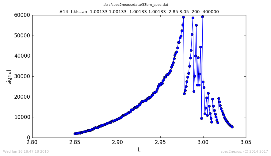
SPEC hklscan (lscan), plotted against L
Get xy data from HDF5 file
One example of complexity is when SPEC has been used to direct data collection but the data is not stored in the SPEC data file. The SPEC data file scan must provide some indication about where the collected scan data has been stored.
The USAXS instrument at APS has a FlyScan macro that commands the instrument to collect data continuously over the desired \(Q\) range. The data is written to a NeXus HDF5 data file. Later, a data reduction process converts the arrays of raw data to one-dimensional \(I(Q)\) profiles. The best representation of this reduced data is on a log-log plot to reveal the many decades of both \(I\) and \(Q\) covered by the measurement.
With the default handling by LinePlotter, no plot
can be generated since the dfata is given in a separate HDF5 file. That file
is read with the custom handling of the usaxs_flyscan.py demo:
usaxs_flyscan.py example
1 2 3 4 5 6 7 8 9 10 11 12 13 14 15 16 17 18 19 20 21 22 23 24 25 26 27 28 29 30 31 32 33 34 35 36 37 38 39 40 41 42 43 44 45 46 47 48 49 50 51 52 53 54 55 56 57 58 59 60 61 62 63 64 65 66 67 68 69 70 71 72 73 74 75 76 77 78 79 80 81 82 83 84 85 86 87 88 89 90 91 92 93 94 95 96 97 98 99 100 101 102 103 104 105 106 107 108 109 110 111 112 113 114 115 116 117 118 119 120 121 122 123 124 125 126 127 128 129 130 131 132 133 134 135 136 137 138 139 140 141 142 143 144 145 146 147 148 149 150 151 | #!/usr/bin/env python
#-----------------------------------------------------------------------------
# :author: Pete R. Jemian
# :email: prjemian@gmail.com
# :copyright: (c) 2014-2017, Pete R. Jemian
#
# Distributed under the terms of the Creative Commons Attribution 4.0 International Public License.
#
# The full license is in the file LICENSE.txt, distributed with this software.
#-----------------------------------------------------------------------------
'''
Plot data from the USAXS FlyScan macro
.. autosummary::
~read_reduced_fly_scan_file
~retrieve_flyScanData
~USAXS_FlyScan_Structure
~USAXS_FlyScan_Plotter
'''
import h5py
import numpy
import os
import spec2nexus.specplot
import spec2nexus.specplot_gallery
# methods picked (& modified) from the USAXS livedata project
def read_reduced_fly_scan_file(hdf5_file_name):
'''
read any and all reduced data from the HDF5 file, return in a dictionary
dictionary = {
'full': dict(Q, R, R_max, ar, fwhm, centroid)
'250': dict(Q, R, dR)
'5000': dict(Q, R, dR)
}
'''
reduced = {}
hdf = h5py.File(hdf5_file_name, 'r')
entry = hdf['/entry']
for key in entry.keys():
if key.startswith('flyScan_reduced_'):
nxdata = entry[key]
d = {}
for dsname in ['Q', 'R']:
if dsname in nxdata:
value = nxdata[dsname]
if value.size == 1:
d[dsname] = float(value[0])
else:
d[dsname] = numpy.array(value)
reduced[key[len('flyScan_reduced_'):]] = d
hdf.close()
return reduced
# $URL: https://subversion.xray.aps.anl.gov/small_angle/USAXS/livedata/specplot.py $
REDUCED_FLY_SCAN_BINS = 250 # the default
def retrieve_flyScanData(scan):
'''retrieve reduced, rebinned data from USAXS Fly Scans'''
path = os.path.dirname(scan.header.parent.fileName)
key_string = 'FlyScan file name = '
comment = scan.comments[2]
index = comment.find(key_string) + len(key_string)
hdf_file_name = comment[index:-1]
abs_file = os.path.abspath(os.path.join(path, hdf_file_name))
plotData = {}
if os.path.exists(abs_file):
reduced = read_reduced_fly_scan_file(abs_file)
s_num_bins = str(REDUCED_FLY_SCAN_BINS)
choice = reduced.get(s_num_bins) or reduced.get('full')
if choice is not None:
plotData = {axis: choice[axis] for axis in 'Q R'.split()}
return plotData
class USAXS_FlyScan_Plotter(spec2nexus.specplot.LinePlotter):
'''
customize `FlyScan` handling, plot :math:`log(I)` *vs.* :math:`log(Q)`
The USAXS FlyScan data is stored in a NeXus HDF5 file in a subdirectory
below the SPEC data file. This code uses existing code from the
USAXS instrument to read that file.
'''
def retrieve_plot_data(self):
'''retrieve reduced data from the FlyScan's HDF5 file'''
# get the data from the HDF5 file
fly_data = retrieve_flyScanData(self.scan)
if len(fly_data) != 2:
raise spec2nexus.specplot.NoDataToPlot(str(self.scan))
self.signal = 'R'
self.axes = ['Q',]
self.data = fly_data
# customize the plot just a bit
# sample name as given by the user?
subtitle = '#' + str(self.scan.scanNum)
subtitle += ' FlyScan: ' + self.scan.comments[0]
self.set_plot_subtitle(subtitle)
self.set_x_log(True)
self.set_y_log(True)
self.set_x_title(r'$|\vec{Q}|, 1/\AA$')
self.set_y_title(r'USAXS $R(|\vec{Q}|)$, a.u.')
def plottable(self):
'''
can this data be plotted as expected?
'''
if self.signal in self.data:
signal = self.data[self.signal]
if signal is not None and len(signal) > 0 and len(self.axes) == 1:
if len(signal) == len(self.data[self.axes[0]]):
return True
return False
def debugging_setup():
import sys
import shutil
sys.path.insert(0, os.path.join('..', 'src'))
path = '__usaxs__'
shutil.rmtree(path, ignore_errors=True)
os.mkdir(path)
sys.argv.append('-d')
sys.argv.append(path)
sys.argv.append(os.path.join('..', 'src', 'spec2nexus', 'data', '02_03_setup.dat'))
def main():
selector = spec2nexus.specplot.Selector()
selector.add('FlyScan', USAXS_FlyScan_Plotter)
spec2nexus.specplot_gallery.main()
if __name__ == '__main__':
# debugging_setup()
main()
|
The data is then rendered in a customized log-log plot of \(I(Q)\):
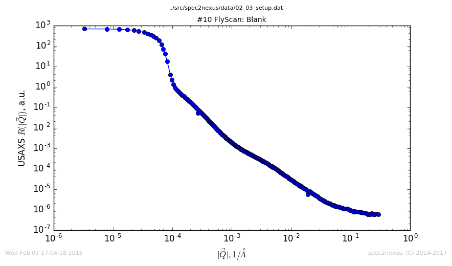
USAXS FlyScan, handled by USAXS_FlyScan_Plotter
Usage
When a custom scan macro handler is written and installed using code similar to the custom ascan handling above:
def main():
    selector = spec2nexus.specplot.Selector()
    selector.add('ascan', Custom_Ascan)
    spec2nexus.specplot_gallery.main()


if __name__ == '__main__':
    main()
then the command line arugment handling from spec2nexus.specplot_gallery.main()
can be accessed from the command line for help and usage information.
Usage:
user@localhost ~/.../spec2nexus/demo $ ./ascan.py
usage: ascan.py [-h] [-r] [-d DIR] paths [paths ...]
ascan.py: error: too few arguments
Help:
user@localhost ~/.../spec2nexus/demo $ ./ascan.py -h
usage: ascan.py [-h] [-r] [-d DIR] paths [paths ...]

read a list of SPEC data files (or directories) and plot images of all scans

positional arguments:
  paths              SPEC data file name(s) or directory(s) with SPEC data
                     files

optional arguments:
  -h, --help         show this help message and exit
  -r                 sort images from each data file in reverse chronolgical
                     order
  -d DIR, --dir DIR  base directory for output (default:/home/prjemian/Documen
                     ts/eclipse/spec2nexus/demo)